detection engineering: understanding alert capacity

why

My last post claimed that 3 things matter in a detection engineering program: coverage, quality, and capacity. In this post I want to spend some time exploring the last in more detail. Specifically, I want to introduce a method that can help us answer common questions that come up in this space. Some examples include:

• What total alert rate can the triage team handle?
• What expected alert rate is reasonable for deploying a new rule?
• What alert rate for an existing rule should trigger a review?
• How many triage analysts do we need?
• What is the payoff for automation?

Having answers to these questions is important. A given capacity imposes an alert budget and there are material consequences to exceeding it. Examples include operational burnout, reduced efficacy and efficiency, and even complete functional collapse. While it is easy to handwave answers, we can do a lot better with a little effort.

Intuitively, a higher capacity leads to better outcomes with respect to our stated purpose:

To continuously convert threat knowledge into signals that reveal adversary behaviour in your environment and enable the timely disruption of their progress toward malicious goals.

All else being equal, the ability to handle a higher alert rate leads to:

1. Lower alert wait time.
2. Lower time to disposition.
3. Lower time to containment.
4. Higher probability of successful adversary disruption.

But how do we know what our current capacity is? How do we know if we are under or over budget, and by how much? How can we know the impact of changing factors that affect it?

Like quality, capacity is somewhat complex and there are many contributing factors. These include:

• The number of analysts you have.
• The experience, expertise, and motivation of your analysts.
• The maturity of your triage processes.
• The analysis tools available.
• How much of your alert triage and response is automated.

In practice, we can approach this in many ways. The approach I want to illustrate here is modelling. Note, all slopped calculator and plotting code used can be found here.

model one

Let’s start simple by trying to answer the following question:

What maximum alert rate $C$ can the triage team handle?

Before we go further, we have to define what we mean by handle. For now, let’s say that it means the queue (backlog of alerts) doesn’t continue to grow forever.

As a first attempt, let’s say $C$ is the product of the number of triage analysts, $c$, and the average rate that they can disposition alerts, $\mu$. So $$ C = c\mu $$ As an example, if there are $c=5$ triage analysts and they can each close $\mu=2$ alerts per hour on average, then $C=10$ alerts per hour. If the arrival rate of alerts, $\lambda$, exceeds 10, then your queue is unstable. Utilisation exceeds 100% and the number of alerts in the queue grows indefinitely. In fact, as $\lambda$ approaches 10, triage analysts lose time for non-triage work. They can’t attend meetings, do admin, or uplift through continuous improvement. The stability of the system depends on the condition $$\rho = \frac{\lambda}{c\mu} < 1$$ This model is simple and it can answer our question. It can also answer other questions we raised. From the resourcing perspective, given $\mu$ and $\lambda$, we can work out the minimum number of analysts we need for stability, $c$. Additionally, $\rho$ also tells us the average utilisation of our triage analysts. An important consideration for ensuring sufficient time can be allocated to non-triage work. Things start to get a bit tricky though if we change our definition of handle.

In detection and response, speed matters. We are usually the last line of defence. By the time an event turns into an alert, the task is to limit impact. To that end, we try to measure our ability to limit impact by imposing time-based response goals. Examples might sound like:

• 90% of alerts acknowledged within 15 minutes or
• 80% of alerts dispositioned within 60 minutes.

Alert arrivals and handling times are somewhat stochastic. This model doesn’t capture the variability. Outside long term stability and utilisation, it isn’t equipped to tell us about the probabilistic properties of the queue. Our response goals are examples of such properties.

model two

Enter queueing theory. Let’s suppose that:

1. A Poisson process describes the arrival of alerts, so the time between alerts is exponentially distributed with arrival rate $\lambda$.
2. Triage times are exponentially distributed, with rate $\mu$.

These conditions define the $M/M/c$ queue, a multi-server queueing model. The first and second $M$ signify that the time between arrivals and service times are Markovian. This is equivalent to what we stated in suppositions 1 and 2. The $c$ means $c$ servers. The same stability condition applies to this model $$\rho = \frac{\lambda}{c\mu} < 1$$ $\rho$ also tells us the average utilisation of our triage analysts. If this condition holds, we can derive many interesting properties of the queue. I will skip overly lengthy derivations here. But you can find them in standard textbooks. As an example, the probability that an alert will need to wait in the queue is given by $$ \text{P}(T_w > 0) = \frac{1}{1+(1-\rho)\left(\frac{c!}{(c\rho)^c}\right)\sum_{k=0}^{c-1} \frac{(c\rho)^k}{k!}} $$ This is known as Erlang’s C formula. To investigate a time-based acknowledgement goal, we want to know the probability that an alert waits less than a threshold $t > 0$ $$\text{P}(T_w < t)$$ This can happen in two ways, either the alert does or doesn’t wait $$ \text{P}(T_w = 0)\text{P}(T_w < t \mid T_w = 0) + \text{P}(T_w > 0)\text{P}(T_w < t \mid T_w > 0) $$ Working through this expression to known quantities:

1. Using the law of total probability, $\text{P}(T_w = 0) = 1 - \text{P}(T_w > 0)$. The right hand side we can evaluate since we have an expression already for $\text{P}(T_w > 0)$ in terms of the model parameters.
2. Conditioning on $T_w = 0$, the probability an alert waits less than $t$ is clearly 1, so $\text{P}(T_w < t \mid T_w = 0) = 1$.
3. If an alert has to wait, then the waiting time distribution is exponential with rate $c\mu - \lambda$. So the conditional cumulative distribution function is given by $$ \text{P}(T_w < t \mid T_w > 0) = 1 - e^{-(c\mu-\lambda)t} $$

The simplified expression for looking at acknowledgement is then $$ \text{P}(T_w < t) = 1 - \text{P}(T_w > 0) e^{-(c\mu-\lambda)t} $$ Let’s try this with 90% of alerts acknowledged within 15 minutes where $c=5$ and $\mu=2$. The capacity is

$ ./cli.py solve-ack --target 0.9 --t 0.25 --mu 2 --c 5
6.184327488935709

We can also see what the average utilisation is

$ ./cli.py rho --lam 6.184327488935709 --mu 2 --c 5
0.6184327488935709

This means that on average, triage analysts spend roughly ~62% of their time on triage. We can infer that the alert queue must be empty for a significant proportion of time.

What happens to the target if we increase the alert rate to 7, above the capacity?

$ ./cli.py ack --lam 7 --mu 2 --c 5 --t 0.25
0.82152185936068
$ ./cli.py rho --lam 7 --mu 2 --c 5
0.7

Our 90% drops to ~82% acknowledged within 15 minutes and utilisation increases from ~62% to 70%. We can graph this expression to visualise what happens under different scenarios as we alter parameters. Below we can see:

1. The impact of varying $c$ and $\lambda$ on the acknowledgement target.
2. The impact of varying $c$ and $\lambda$ on utilisation.

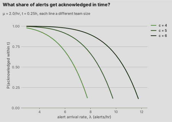
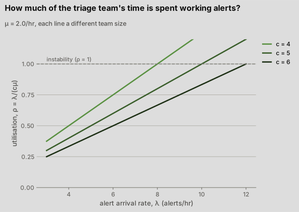
The proportion of alerts acknowledged on time starts to drastically decrease when average utilisation exceeds ~70%. This spare capacity seems to be an integral part of handling variability in the queue behaviour. In particular, surges.

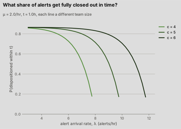
With some extra work we can get to an expression that lets us investigate disposition oriented goals like % of alerts dispositioned within threshold. This case is effectively the same as acknowledgement but we add queue time and handling time. $$ \text{P}(T_d < t) = 1 - \left[ 1 + \frac{\text{P}(T_w > 0) \mu}{(c-1)\mu -\lambda }\right] e^{-\mu t} + \left[ \frac{\text{P}(T_w > 0) \mu}{(c-1)\mu -\lambda } \right] e^{-(c\mu - \lambda) t} $$ This expression has a singularity when $\lambda = (c-1)\mu$. We can remove it by taking a limit to get the special case $$ \text{P}(T_d < t) = 1 - \left( 1 + \text{P}(T_w > 0) \mu t \right) e^{-\mu t} $$

Let’s test this with the same model parameters we used before. We want 80% of alerts dispositioned within 60 minutes, so the alert capacity is

$ ./cli.py solve-disposition --target 0.8 --t 1 --mu 2 --c 5
7.000330535702345

This is a higher capacity than our acknowledgement target allowed. Under these conditions, the disposition target is slightly more relaxed. Below we can see the impact of varying $c$ and $\lambda$ on the disposition target

Now that we have a model that can help us answer important and interesting questions about alert capacity, how does it go wrong? Well, many of the assumptions made by the model don’t hold in practice. Some examples are listed below.

• Alerts are handled FIFO In practice, alerts are probably not handled FIFO. In fact, a prioritisation system effectively partitions a single queue into multiple queues. You attend to priority alerts before you attend to low priority alerts. Low priority alerts need to wait until the queue is empty of high priority alerts, regardless of the arrival order.
• The triage team operates 24/7 A full 24/7 triage team is disproportionately resource intensive compared to other common staffing models. Alternatives include 8x5, 12x5, or 12x7 with augmentation through on-call or outsourcing during non-core hours. If you deploy an alternate staffing model, $c$ is effectively 0 or at least reduced during non-core hours, or we only triage high priority alerts.
• Alerts arrive independently Events that generate alerts are often not entirely independent. Threat actor campaigns can be coordinated and concentrated in time and multiple alerts can arise from the same underlying activity.
• The arrival rate of alerts is stationary The arrival rate depends on many factors that change in time. Examples include employee activity, attack and detection surfaces, and the threat actor ecosystem. Some of these things are not easily predictable and can be difficult to account for.

I think that in most situations, deviations from assumptions will result in immaterial prediction errors or we can account for them easily. If not, more sophisticated models exist. Examples include $M/G/k$ (where triage time is a general distribution) or $M/M/c$ with priority classes. Alternatively, we can run discrete event simulations to estimate empirical probabilities.